Author: gknow81

Computational Estimation of Magnetic Flux Density for Layered Annular Sector Coils

Building on my first attempt using circular loops, this post details a more refined Python analysis of airgap flux density. This version increases realism by modeling windings as multi-layer annular sectors – a shape better reflecting my design – calculated using the Biot-Savart law. For windings supported by materials like FR4 PCB (µᵣ ≈ 1, similar to air), the Biot-Savart ‘air’ calculation holds well. Consequently, these results should be reasonably close to FEA simulations configured to neglect secondary effects. Finite Element Analysis (FEA) is still the logical progression and my planned next step in evaluating this design.
(The Python notebook can be downloaded at the bottom of the page)

Motivation: Towards Realistic Coil Geometry

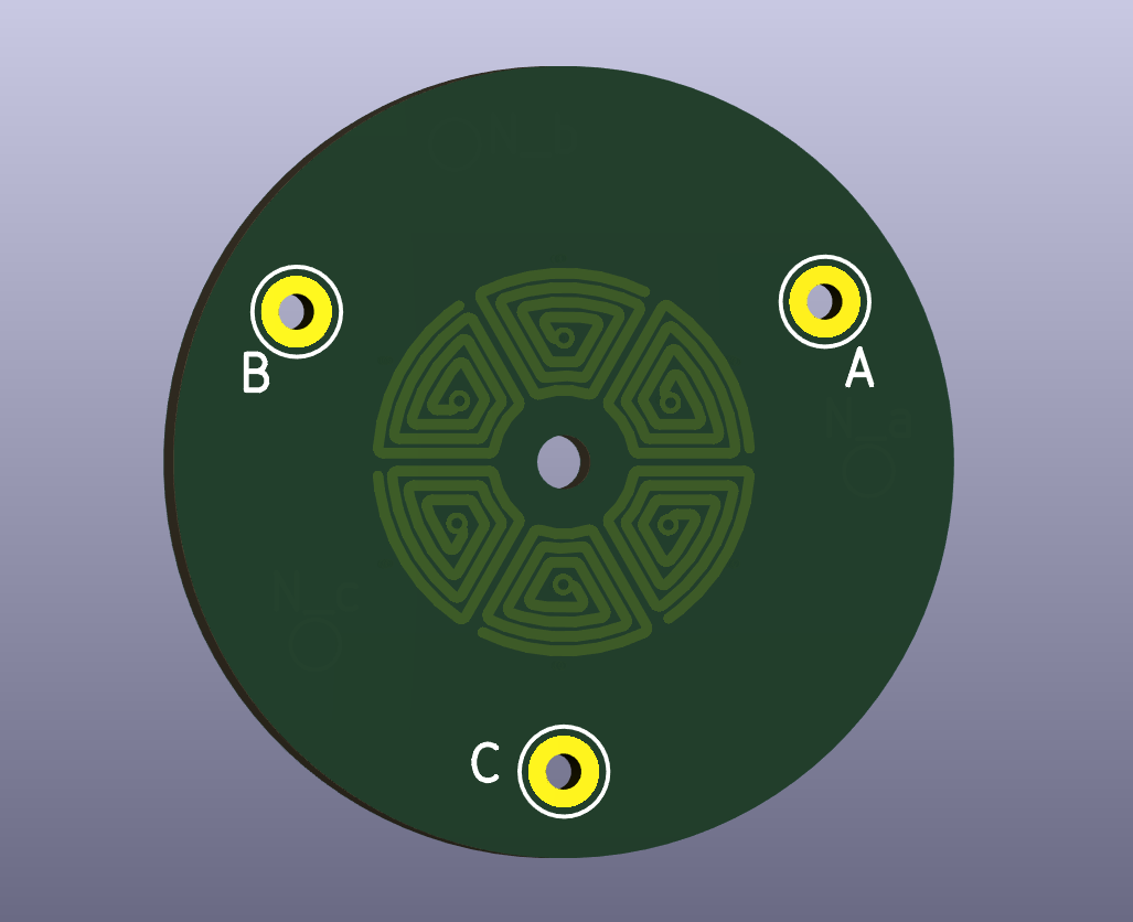
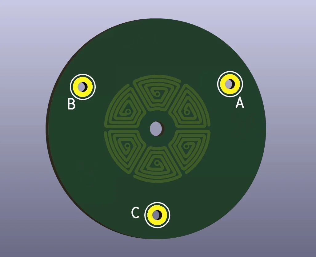
A real motor winding isn’t just a single loop. It consists of multiple turns wound layer upon layer. To capture this more accurately, this simulation models each layer as a series of contracting annular sectors. Imagine starting with the outermost boundary of the coil cross-section and then winding inwards, turn by turn, with a defined spacing. Furthermore, multiple such layers are stacked axially, offset slightly from each other. This approach provides a much better geometric approximation of the actual current distribution compared to a single, simple loop.

The Approach: Iterative Geometry and Grid-Based Biot-Savart

1. Generating the Winding Paths:

   • The core shape is an annular sector (a slice of a doughnut).

   • The create_single_sector_perimeter_angled_closed function generates the points defining the perimeter of one such sector.

   • The key generate_disconnected_loops function takes the initial outer/inner radii and angle and iteratively calculates the geometry for subsequent turns within a layer. It reduces the outer radius and increases the inner radius by the SPIRAL_SPACING for each “turn,” also adjusting the angular width slightly to approximate constant wire width. This continues until the inner and outer radii meet or a maximum loop count (MAX_LOOPS_PER_LAYER) is reached.

   • This process creates a list of 2D loop paths representing the turns within a single layer.

   • Multiple layers are then created by copying this 2D loop list and assigning different Z-coordinates based on NUM_LAYERS and LAYER_OFFSET.

2. Defining the Calculation Space:

   • Instead of calculating the field everywhere (computationally expensive), we define a specific region of interest: the airgap.

   • The annulus_grid_points_xyz_angle function generates a grid of points within an annular sector located at the specified AIRGAP_DISTANCE from the first layer. The density of this grid is controlled by NUM_RADIAL_GRID and NUM_ANGULAR_GRID.

3. Applying Biot-Savart:

   • The standard biot_savart_segment_at_point function remains the workhorse. It calculates the infinitesimal magnetic field vector (dB) produced by a short, straight segment of current-carrying wire (dl_vec) at a specific point in space (point).

   • The main calculation loop iterates through every point in the airgap grid.

   • For each airgap point, it then iterates through every segment of every loop in every layer.

   • It calls biot_savart_segment_at_point for each segment and sums up all the resulting dB vectors to get the total magnetic field vector B = (Bx, By, Bz) at that specific airgap grid point.

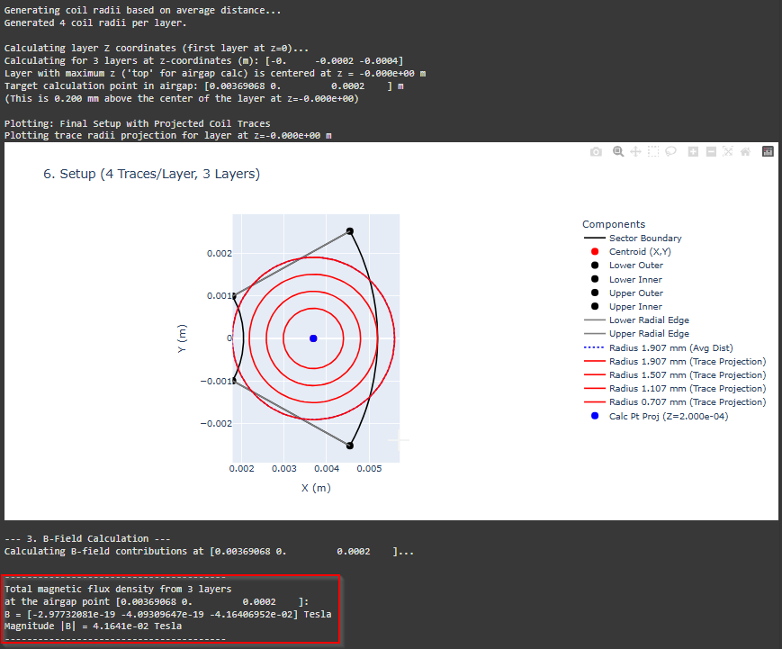
Visualization and Results:

The script generates three key visualizations:

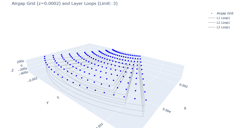
1. 3D Grid & Paths: Shows the physical layout of the multi-layer coil loops (grey lines) and the grid points in the airgap (blue dots) where the field is calculated. This helps verify the geometry setup.

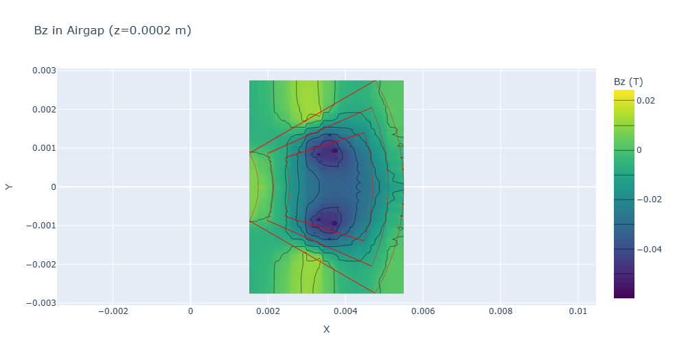
2. Bz Heatmap: Displays the calculated Z-component of the magnetic field (Bz) as a 2D heatmap on the airgap plane. The outlines of the 2D loops are overlaid in red for context. This is often the most critical component for axial flux machine performance.

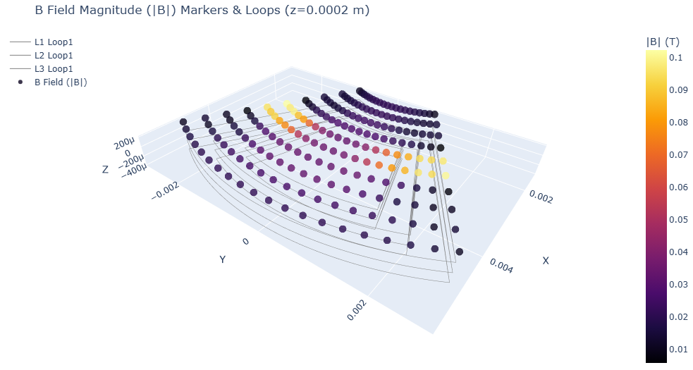
3. B-Field Magnitude Markers: A 3D plot showing the coil loops again, but this time with markers at the airgap grid points. The color of each marker represents the magnitude (|B|) of the magnetic field at that point. (Initially, go.Cone glyphs were used to show direction, but rendering issues with Plotly v6.0.1 when combining many cones and lines necessitated this switch to markers for reliability).

Limitations of the Analytical Approach

While more refined, this model still relies on assumptions and has limitations:

• Idealized Geometry: Assumes perfect annular sectors and uniform current density within wires.

• No Eddy Currents: Doesn’t account for induced currents in conductive materials.

• Computational Cost: Calculating the field from every segment for every grid point can become slow, especially with high point densities or many layers/turns.

Next Steps: Embracing FEA

These limitations highlight why Finite Element Analysis (FEA) is the standard tool for detailed motor design. FEA can:

• Model complex 3D geometries accurately.

• Incorporate non-linear material properties like B-H curves and saturation.

• Calculate eddy currents and other secondary effects.

My next step in this learning journey will be to explore open-source FEA tools (like FEMM for 2D) to model this same axial flux motor configuration and compare the results.

Conclusion and Comparison:

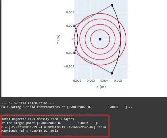
Comparison of magnetic flux density calculations reveals good agreement between the simplified circular estimation and the detailed spatial analysis near the geometric centroid, both yielding approximately 0.04 T. However, the detailed analysis highlights significant spatial variation missed by the simpler model, with flux density increasing to nearly 0.1 T towards the radial edges. The next step will involve Finite Element Analysis (FEA) to provide a more comprehensive simulation and further validate these analytical findings.

(Full Python Notebook will be added in the next 2 days)

Computational Estimation of Magnetic Flux Density for Layered Annular Sector Coils

This post details my vision for a first attempt at estimating the airgap flux density generated by the stator coils in an axial flux motor topology using Python. Future iterations will include a grid-based Biot-Savart approach (calculating the field over an area) and eventually leveraging open-source 2D/3D FEA tools. I know there are many excellent commercial and open-source programs that perform these calculations already, but my primary motivation here was to further understand the underlying physics and calculation methods from first principles, specifically as applied to axial flux machines.
(The Python notebook can be downloaded at the bottom of the page)

This script demonstrates a workflow integrating geometric analysis with fundamental physics:

1. Geometric Foundation: Using numpy, the code precisely defines the 2D cross-section of an annular sector (a “doughnut slice”), representing the physical space for the windings. Parameters like radii and arc angle define the core geometry.

2. Centroid & Characteristic Dimension: The geometric centroid of the sector is calculated. Following this, a characteristic “average distance” from this centroid to the sector’s perimeter is determined. This metric provides a basis for positioning the current elements in the model.

3. Coil Representation & Layering: The core of the model represents the winding pack. Instead of discretizing a potentially complex spiral path, this implementation utilizes concentric circular current loops centered at the geometric centroid.

   • The radii of these loops are derived from the calculated “average distance,” stepping inwards with a defined TRACE_DISTANCE. This structured approach creates a model of the current distribution intended to capture the primary magnetic contributions within the sector.

   • The model effectively handles multiple layers stacked vertically (NUM_LAYERS), incorporating the specified LAYER_SPACING between them.

4. Physics Engine – Biot-Savart Law: The magnetic field calculation leverages the Biot-Savart Law directly. A dedicated function (biot_savart_loop_at_point) numerically integrates the field contributions from infinitesimal current segments (dl) around each modeled circular loop to determine the magnetic field vector (B) produced at any target point in space.

5. Targeted Field Evaluation: The script computes the total B-field by vectorially summing the contributions from all modeled loops across all layers. This calculation is performed at a user-defined point, typically located in the ‘airgap’ region relevant to the device’s operation (e.g., a specific distance above the top layer’s centroid).

6. Visualization with Plotly: Interactive plots generated using plotly are used throughout. They visualize the defined geometry, centroid, average distance metric, the positions of the modeled current loops, and the field evaluation point, providing crucial validation and insight into the model setup.

Advantages of this Method:

• Direct Physics Implementation: Applies the Biot-Savart law directly to the defined current sources, offering a clear link between the model geometry and the resulting field.

• Model Transparency & Control: Python implementation allows full control over the geometric parameters and the current loop representation.

• Computational Speed: For field calculations at specific points arising from known currents in linear media (like air), this direct summation is generally significantly faster than setting up, meshing, and solving a full FEA domain.

• Educational Insight: Provides a practical platform for exploring how different coil parameters and layering strategies influence the magnetic field.

Considerations:

• This method models the current distribution using defined circular elements. It’s most suited for problems where the field is primarily determined by the source currents in air or linear materials.

• It doesn’t inherently include the effects of complex magnetic cores (saturation, hysteresis) or solve for fields within those materials, which are strengths of FEA.

• Consequently, while this direct calculation approach offers compelling speed advantages for rapid estimations, it may not achieve the same level of accuracy as a detailed FEA model, particularly for complex geometries or when material effects are dominant. The trade-off is speed for potentially reduced precision

Code:

Python Notebook Download

Let’s start with a short inductor review:

• Faraday’s Law drives inductors: current through a wire creates a magnetic field.

• The voltage across an inductor is V= L ⋅ (dI/dt), proportional to the rate of current change and inductance (L).

  • Faster current shifts result in a bigger voltage spikes

  • If there is steady current (rate of change is 0), the output voltage from an inductor = 0

  • In the layout of a boost converter the voltage applied to the inductor is equal to the Vin, which results in a linear current rise that builds the magnetic field.

• Typically a coil, an inductor stores energy in its magnetic field, often enhanced by a ferromagnetic core like ferrite—though air-core versions exist too

Boost Converter Design

At work I am used to high-power equipment, so for this boost converter, I chose 5 V in, 12 V out, and 20 A for 240 W of power output. Big designs like this punish sloppy math, and my first attempt proved it. I picked unrealistically tight ripple targets and messed up the input current, using Vout​ in the denominator Vin. This resulted in a on oversized capacitor by a factor of 10, which did not produce a pretty output.

To fix that I used some common percentages—1% voltage ripple (0.12 V), 30% current ripple, and calculated a 53.33 A input current. With 90% efficiency my spice model output came together.

In designing my boost converter circuit, I encountered a few practical challenges that underscored the importance of component selection and compatibility. One oversight occurred when I initially entered the capacitor’s equivalent series resistance (ESR) as 0.02 ohms instead of the intended 0.002 ohms. This seemingly small error significantly amplified the output voltage ripple, as ESR directly influences how effectively the capacitor smooths the boosted voltage. Correcting this brought the ripple under control, but I noticed the average output voltage remained slightly above my 12V target. To address this, I reduced the switch’s duty cycle from 61% to 58%, which aligned the output closer to 12V without noticeably affecting the ripple amplitude.

I was able to reduce the duty cycle partly because I used an inductor larger than the ideal calculated value. A bigger inductor stores more energy in its magnetic field, which let it keep boosting the voltage even with a lower duty cycle. This ties into a core idea with boost converters: you don’t want the inductor’s magnetic field to fully collapse when the switch is off, since it needs enough energy to add to the next cycle to increase the voltage. The output voltage settles when the energy going into the inductor matches what’s delivered to the load and capacitor (minus losses, of course). This shows how critical it is to pick components that work together, especially since the switching frequency heavily influences the inductance needed to avoid dropping into discontinuous mode.

For the diode, I opted for a Schottky type due to its efficiency advantages, well-suited to my moderate output voltage. Unlike traditional PN junction diodes, Schottky diodes feature a metal to N-type semiconductor junction, reducing the forward voltage drop to ~0.3V (vs. 0.7V for PN diodes) and eliminating recovery time by relying solely on majority carriers (electrons). This enables faster switching and lower power losses—critical for a boost converter’s high-frequency operation. The trade-off is an increased reverse leakage current when reverse-biased, due to the reduced Schottky barrier height, though this posed no significant issue for my 12V design. In applications with significantly higher output voltages, however, a different diode or an active switch might be necessary to handle reverse bias conditions.

This experience reinforced how interconnected component choices are in power electronics. From capacitor ESR to inductor sizing and diode characteristics, each decision ripples through the system, shaping efficiency, stability, and performance.

To break down my boost converter’s operation, let’s define two phases: T1, when the switch is on and the inductor current (I_L1​, blue trace) rises, and T2, when the switch is off and the current falls.

T1: Switch On

• During T1, the input voltage (Vin​) drives the inductor (L), causing its current to increase linearly as the magnetic field builds. This follows V = L * (di/dt), visible in the blue trace’s upward slope.

• When the switch is closed, the voltage at the switch node (Vn002​, green trace) falls to near zero because of the minimal resistance in the switch and inductor, while the voltage across the inductor remains equal to Vin.

• Meanwhile, the capacitor (C) sustains the output voltage (Vout​) by supplying current to the load (R).

• You’ll notice a slight dip in the Vout trace, evidence of voltage ripple as the capacitor discharges.

• The diode, reverse-biased here, blocks any backflow from the output to ground, as confirmed by the red trace showing zero diode current.

T2: Switch Off

• When the switch opens in T2, the inductor’s magnetic field collapses, driving current through the diode to the capacitor and load at a steadily declining rate. This induces a voltage across the inductor (V = L * (di/dt)), which adds to Vin to produce the “boosted” Vout​.

• The green trace Vn002​ spikes as the inductor’s voltage reverses polarity (voltage adds to Vin), driving the boost effect. This process transfers energy to the capacitor, which stores it to stabilize Vout​, smoothing the output and supplying current to the load.

• The red trace now shows forward biased diode current flowing, matching the inductor’s discharge.

These phases highlight how the inductor and capacitor work together: L stores energy in T1, then releases it in T2, while C ensures a stable output.

Websites and References Used:

• Boost Converters (Step-Up Converter)

• grok

The purpose of this exercise was to review basic buck converter design. I originally learned this in class at Purdue but have not used it in 4 years and needed a refresher. I will continue this exercise with further reviews on other power converter topologies.

I chose components and a scenario that is maybe not the most elementary buck converter design, but this forced me to consider aspects of design I would have otherwise missed.

With some help from a Texas Instruments PDF and the web, I calculated the Inductor and Output Cap from a parameter list I defined. I approached these parameters with an eMotor/electromagnetic background and intentionally chose a low resistance load.

Next Step was to create a model in LTspice. I started with generic spice components and improvised from there.

The generic components I started with were not working correctly, I believe this was due to the large current draw and low pulse voltage. This led me to find appropriate components for the output current I calculated (33A). I chose a Schottky diode with an average forward current of 40 Amps and 30V breakdown voltage. I then changed to an N-type mosfet with a 42A continuous current rating. These component changes with an extended simulation window to overcome the transient time for the large passive components finally gave me some results close to what I was looking for.

As you can see above, the transient is pretty long, around 60-70ms. This was expected with a 10mF cap and 2.2mH inductor on the output. There could be controls or design changes implemented depending on the use cases to help mitigate this transient time.

From my estimations, the efficiency at this operating point is around 82.5%. I started out by calculating a duty cycle with an assumption of 90% efficiency, the output was around 3.0V. I manually adjusted the “Ton” parameter of the gate driver to achieve the desired output of 3.3V. The duty cycle that achieved 3.3V was 80%. I then plugged this back into the duty cycle equation and solved for the efficiency parameter. In ideal calculations it would be 66%, which highlights the inefficiencies of this design. My assumptions are that these losses mainly come from the switch and diode.

I plan to revisit this design and try implementing improvements to increase efficiency. This would include plotting the losses on the diode vs the MOSFET at different duty cycles and evaluating the effect of replacing the diode with a switch. It might come down to needing a more efficient MOSFET with a lower Rds(on).

Websites and documents used:

• Monolithicpower.com

• ti.com

A quick intro to the project:
This is a personal project inspired by my opinions on the future of electric motors and their use cases. I believe that we need to continue to find ways to make motors smaller, lighter, more power dense, and easier to manufacture all while simplifying the number of subcomponents. This will benefit every industry, but my specific focus is robotics and drones. In the future, these items will be mass produced at volumes far beyond almost any other electric motor use case, therefore every pound, penny, and second count!

I started working on this in late January of this year (2025) and conducted research, wrote analytical analysis scripts, and designed a prototype. The first prototypes were ordered at the beginning of March and I expect to begin proof of concept and functional testing as soon as they arrive.

If all goes well, I plan to try and patent aspects of my design at somepoint. For this reason, I will not share all the details on the design and operation.

I will make more detailed posts on this project in the coming weeks/months, please come back every so often to check for updates!

Below is an image of the stator prototype I just sent for manufacturing.

Throughout winter and summer 2024, I completed the Post Graduate Program in AI and Machine Learning: Business Applications from UT Austin. The 6-month program provided valuable insights into Python use cases, machine learning, and LLM applications. The number of opportunities and the level of freedom afforded by open source and Python was an eye-opening experience. All class modules included lectures, quizzes, hands-on application through mentored learning sessions, and an implementation project.

The following sections were covered in the class:

Module 1: Python Foundations
Module 2: Machine Learning
Module 3: Advanced Machine Learning
Module 4: Neural Networks
Module 5: Computer Vision
Module 6: Natural Language Processing

To keep things concise, I will post my Google Collab python projects (Google’s version of jupyter notebooks) below as html downloads:

• Project01_FoodHub

• Project02_PersonalLoanCampaign

• Project03_CCUsersChurn

• Project04_BankChurnPrediction

• Project05_SeedlingClassification

• Project06_SupportTicketCategorization

Certificate of Completion: